Plotting & rich output

A fit result is only as useful as the picture you can draw from it. NativeMinuit gives you three layers, from "just call plot" to "drop a table into a paper":

1. Plot recipes — plot(result) on any result type, as backend-agnostic RecipesBase recipes rendered via Plots.jl.
2. iminuit-style draw_* helpers — the familiar draw_contour / draw_mnprofile / draw_mnmatrix family from IMinuit.jl / iminuit, returning a Plots.Plot.
3. Rich text output — a fitted Minuit auto-renders as an HTML table in Jupyter and a Unicode box in the REPL; to_latex gives a publication table and mn_plot_text an ASCII plot for headless runs.

Which to reach for: use a recipe (plot(x)) when you have a result object in hand and want the obvious picture; use a draw_* helper when you are porting IMinuit.jl code or want the iminuit-named entry point that builds the scan for you; use the rich output for reports, papers, and terminals.

Plot recipes — plot(result)

Every visible result type ships a RecipesBase recipe. RecipesBase is backend-agnostic in principle, but the path that ships and is exercised is Plots.jl — load it and pick a backend as usual (NativeMinuit itself depends on no plotting package):

using NativeMinuit, Plots
gr()                           # or plotlyjs(), etc.

Fit results, errors, contours

There is no recipe for Minuit itself — plot the underlying FunctionMinimum via m.fmin. Likewise minos!/minos mutate m and return it (not a MinosError), so run MINOS first, then plot the stored MinosError objects from m.merrors:

m = Minuit(cost, x0); migrad!(m)

plot(m.fmin)                              # parameter values with Hesse error bars
minos!(m)                                 # run MINOS, fills m.merrors
plot(collect(values(m.merrors)))          # Vector{MinosError} → multi-parameter error bars
plot(m.merrors["a"])                      # a single MinosError → one asymmetric error bar
plot(contour_ellipse(m, 1, 2))            # ContoursError → closed 1σ contour polygon
plot(contour_grid(m, 1, 2))               # ContourGrid → filled FCN-landscape contour

The recipes attach sensible defaults (markers, labels, aspect_ratio for the contour) and pass through any plot keyword.

A worked example — a two-parameter linear fit, its Hesse error bars, and the exact joint 68 % confidence contour (both blocks share the fitted m):

using NativeMinuit, Plots, Random
gr()                                            # headless-friendly backend
Random.seed!(1)
xs = range(0, 1; length = 30); σ = 0.1
ys = 0.5 .+ 2.0 .* xs .+ σ .* randn(30)
χ²(p) = sum(((ys .- (p[1] .+ p[2] .* xs)) ./ σ) .^ 2)
m = Minuit(χ², [0.0, 0.0]; names = ["a", "b"]); migrad!(m); hesse!(m)
plot(m.fmin)                                    # value ± Hesse error bars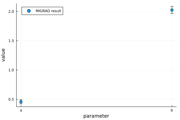

draw_mncontour(m, 1, 2; numpoints = 50)         # exact joint 68 % confidence contour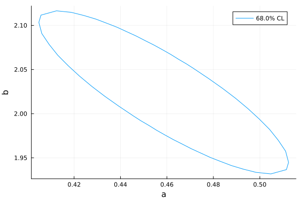

Error-analysis results

The error-analysis outputs from the Error analysis page each have a recipe too. A parameter pair is selected with the vars option (two indices or names; default the first two free parameters), a single parameter with par (an index or name; default the first varying parameter).

# MC-Δχ² sample cloud: 2D scatter of the accepted set, coloured by Δχ².
r = get_contours_samples(m; nsamples = 20_000, cl = 1, seed = 1)
plot(r)                          # first two free parameters
plot(r; vars = ("mass", "g"))    # pick the pair by name

# Bootstrap / jackknife: histogram of one parameter's resampled distribution,
# with the estimate and the CI / jackknife-mean drawn as reference lines.
# Its asymmetry about the estimate is exactly what a symmetric error bar hides.
plot(bootstrap(model, data, m; nresample = 2000, seed = 1))   # first free par
plot(jackknife(model, data, m); par = "k")

# Multi-modal solutions: one colour per cluster, each representative starred.
S     = r.samples
modes = find_solution_modes(S, m)
plot(modes, S)                   # cluster the point cloud (pass the same matrix)
plot(modes)                      # no samples → per-mode bounding boxes + reps
plot(modes; vars = (1, 3))       # project onto a chosen parameter pair

vars / par are recipe-only options consumed before the backend sees them, so they never trigger an "unsupported attribute" warning.

For instance, the MC-Δχ² accepted cloud of the fit above, each point coloured by its Δχ²:

r = get_contours_samples(m; nsamples = 4000, cl = 1, seed = 1)
plot(r)                          # 2D scatter over the accepted Δχ² ≤ 1 region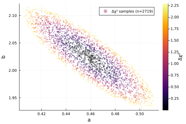

iminuit-style draw_* helpers

These mirror IMinuit.jl's / iminuit's m.draw_* methods: each takes a fitted Minuit, builds the scan/contour for you, and returns a Plots.Plot. They are Plots.jl-based — load using Plots to enable them (they live in a package extension that activates automatically). They are bare stubs with no fallback, so calling one before using Plots raises a MethodError. (By contrast, optim / minimize_with dispatch through Base.get_extension, so calling those without Optim raises a friendly "load Optim.jl" message instead.)

using NativeMinuit, Plots
m = Minuit(cost, x0); migrad!(m)

draw_contour(m, 1, 2)             # FCN grid-slice landscape (filled contour)
draw_mncontour(m, 1, 2)           # exact joint 68% confidence contour
draw_mncontour(m, 1, 2; cl = [0.68, 0.95])  # overlay several CLs
draw_profile(m, 1)                # 1D scan along par 1 (no inner minimisation)
draw_mnprofile(m, 1)              # 1D MINOS profile (re-minimise the rest)
draw_mnmatrix(m)                  # triangular matrix of all pairwise MINOS contours

par is a 1-based index or a parameter-name string, and trailing kws... flow through to the underlying Plots.plot.

For the IMinuit.jl data-and-fit scatter macros — @plt_data, @plt_data!, @plt_best, @plt_best! — see the Data / model_fit workflow; they likewise expand to Plots.scatter(...) and need using Plots in scope.

Rich text output

A fitted Minuit knows how to display itself in three formats.

Jupyter / Pluto (HTML) and the REPL (Unicode)

No call is needed — show does it. In a Jupyter or Pluto notebook a fitted Minuit renders as an HTML table: a merged value ± Hesse-error column before MINOS, widening after minos! into side-by-side Value, Hesse and MINOS columns (a MINOS side that failed to converge is marked invalid, so a one-sided MINOS still shows the side it got; — means MINOS was not run for that parameter), a χ²/ndf and p-value header for a χ² fit, a per-flag validity checklist, and a colour correlation-matrix heatmap with a near-degeneracy warning for strongly-correlated pairs. In the REPL the same information prints as a Unicode box:

m = Minuit(cost, x0); migrad!(m); minos!(m)
m                       # rich auto-display (HTML in Jupyter, box in the REPL)

The result types also self-render in the REPL: FunctionMinimum, BoundedFunctionMinimum, and MinosError (and a Vector{MinosError}) each print their own Unicode summary box.

LaTeX table — to_latex

to_latex renders the fitted parameters as a publication-ready LaTeX table, numbers already rounded to the uncertainty (1–2 significant figures on the error, value to match):

print(to_latex(m))                                  # booktabs + siunitx \num{}
print(to_latex(m; siunitx = false, booktabs = false))  # plain numbers, \hline
print(to_latex(m; caption = "Fit result", label = "tab:fit"))  # wrap in a float

Defaults to a booktabs rule set with siunitx \num{} numbers (so the preamble needs \usepackage{booktabs} and \usepackage{siunitx} unless you disable them). Asymmetric MINOS errors are written \num{x}^{+hi}_{-lo}, a symmetric Hesse error as \num{x} \pm \num{e}, and a fixed parameter as the bare value tagged (fixed).

A second method renders a single MinosError as inline math (\num{value}^{+hi}_{-lo}, no surrounding $…$) for dropping into running text:

minos!(m, 1)                     # run MINOS so the asymmetric error exists
to_latex(m.merrors["a"])         # a MinosError → e.g. "\\num{1.23}^{+0.05}_{-0.04}"

(minos(m, 1) / minos!(m, 1) return the mutated Minuit, not a MinosError — fetch the error from m.merrors[name] or m.minos_errors[index].)

ASCII plot — mn_plot_text

For a headless run (CI, an SSH session, a log file) where no plotting backend is available, mn_plot_text renders a 2D point set as a Cartesian box of characters and returns a String ready for println / @info:

# An (ellipse-approximation) contour as ASCII (the minimum is marked X):
println(mn_plot_text(contour_ellipse(m, 1, 2; npoints = 24)))

# Or any raw vector of (x, y) points (e.g. from mncontour):
pts = mncontour(m, 1, 2)
println(mn_plot_text(pts; par_x = "mass", par_y = "g", width = 50, height = 16))

The box auto-scales to the data and snaps to round-number ticks (the Minuit2 mnbins heuristic), so width / height are hints. A single point is *, an overlap of differing characters is &, and a supplied centre is X. An invalid or empty input renders an explanatory message rather than throwing.

See also

• Error analysis — the sampling / resampling / multimodal results whose recipes are shown above.
• Recipes implementation: src/plot_recipes.jl; draw_* extension ext/NativeMinuitPlotsExt.jl.
• Rich output: src/display.jl (to_latex), src/plot_text.jl (mn_plot_text).